Example data: steel frame with 3D scanning laser vibrometer#
All example scripts and notebooks in the scripts/ directory use the same
measurement dataset, included in the repository under tests/files/.
This page describes the test structure, the 3D laser vibrometer measurement
technique, and the multi-setup scan arrangement.
Test structure#
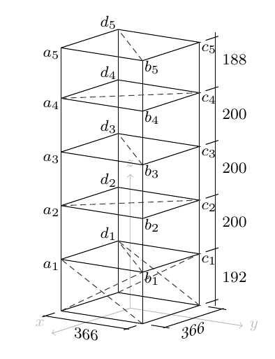
Steel-frame test structure with axis/floor labelling (axes a–d, floors 1–5).#
The test object is a slender steel-frame skeleton at the Institute of Structural Mechanics (ISM), Bauhaus-Universität Weimar:
Height: approx. 1 m
Base footprint: 36 cm × 36 cm (square)
Columns: four threaded rods M8 steel, one at each corner
Floors: five horizontal platforms, each made of several 5 mm steel plates bolted between pairs of hex nuts — effectively clamped to the columns at each level
Boundary condition: the lowest floor is bolted rigidly to a heavy wooden base plate (fixed-base condition)
The node labels follow the thesis convention: axis (a–d) × floor (1–5),
e.g. a1 to c5, and d5. The grid.txt file uses a
corresponding numbering scheme (nodes 1–24):
Level |
z (cm) |
Nodes |
|---|---|---|
0 |
0 |
1 – 4 (base, fixed) |
1 |
19.2 |
5 – 8 |
2 |
39.2 |
9 – 12 |
3 |
59.2 |
13 – 16 |
4 |
79.2 |
17 – 20 |
5 |
98.0 |
21 – 24 |
Within each level the four nodes sit at the corners of the 36 cm × 36 cm square (x, y = ±18.1 cm). Node 24 (top of the far corner, axis d, floor 5) is the permanent reference location.
Asymmetric cross-bracing is fitted at the lowest level in the y-direction only, which separates the first bending modes in x and y and avoids degenerate (coupled) mode pairs. The structure exhibits at least eight clearly identifiable vibration modes below 15 Hz: first and second bending in x and y, first and second torsion, and a longitudinal mode.
Ambient excitation#
The structure was excited by two electric fans placed on either side, providing broadband aerodynamic (output-only) excitation. No force measurement was made — the classical OMA scenario.
3D scanning laser vibrometer#
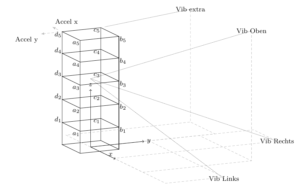
Arrangement of the three PSV 400-3D scan heads (left, right, top) and the accelerometer reference sensors at node d5.#
The measurements were performed with a Polytec PSV 400-3D system: three scanning laser Doppler vibrometer (LDV) heads, each independently steerable.
Measurement principle#
A laser Doppler vibrometer measures instantaneous vibration velocity by detecting the Doppler frequency shift of the laser light reflected from a moving surface. Because the Doppler shift is caused only by the component of velocity along the beam axis, each head measures only the projection of the true 3-D vibration vector onto its own beam direction:
where e is the unit vector along the beam, α is the azimuth and β is the elevation angle. With three heads aimed from different directions, the three simultaneous measurements form a system of equations that can be solved for the three Cartesian velocity components — provided the beams are not coplanar.
Skewed (oblique) measurement directions#
In the dataset the three heads are positioned in front of the structure so that beams converge approximately on each measurement node. Because the heads are at a finite distance and offset to the sides and above, all beams arrive at oblique angles — none of the three coincides with a global Cartesian axis:
Channel |
Azimuth (approx.) |
Elevation (approx.) |
|---|---|---|
vib_l (left head) |
15 – 29 ° |
−18 – −9 ° |
vib_r (right head) |
79 – 81 ° |
−17 – −7 ° |
vib_t (top head) |
46 – 56 ° |
+28 – +35 ° |
The exact angles for each setup and node are stored in the per-setup
channel_dofs.txt file and are read by
PreProcessSignals via the chan_dofs
attribute. They are later used by
ModeShapePlot to project the identified mode
shapes from the oblique measurement coordinate system back to global Cartesian
for visualisation.
Note
In OMA you do not need to transform time series to orthogonal Cartesian coordinates before system identification. Identification operates on the oblique (laser-direction) channels directly. The transformation to x/y/z happens afterwards during mode-shape post-processing using the stored azimuth/elevation angles.
Reference sensors#
Two piezoelectric accelerometers are permanently mounted on node 24 (d5, the highest corner of the back column) and are oriented along the global x and y axes. They serve as fixed reference channels across all 15 setups, enabling PoSER and PoGER merging:
Channel 3 — accelerometer, node 24, x-direction (azimuth 0°, elevation 180°)
Channel 4 — accelerometer, node 24, y-direction (azimuth −90°, elevation 0°)
Channel 5 — accelerometer, node 24, z-direction — present in raw data but excluded from the analysis (
Delete Channels: 5insetup_info.txt)
Multi-setup scan arrangement#
The 3D-SLDV scans one node at a time: all three laser heads point simultaneously at a single node, record for the measurement duration, then the heads are re-aimed at the next node. The complete dataset covers 15 setups, scanning nodes 5 – 19 (floors 1 – 4) in sequence:
Setup |
Node |
Active rover channels |
Floor / height |
|---|---|---|---|
1 |
5 |
vib_l, vib_r, vib_t (+ ref_x, ref_y) |
Floor 1 / 19.2 cm |
2 |
6 |
vib_l, vib_r, vib_t (+ ref_x, ref_y) |
Floor 1 / 19.2 cm |
3 |
7 |
vib_l, vib_r, vib_t (+ ref_x, ref_y) |
Floor 1 / 19.2 cm |
… |
… |
… |
… |
15 |
19 |
vib_l, vib_r, vib_t (+ ref_x, ref_y) |
Floor 4 / 79.2 cm |
Each setup directory tests/files/measurement_<n>/ contains:
measurement_<n>.npy— raw time series, shape (n_samples × 6), columns 0–5setup_info.txt— sampling rate (256 Hz), reference channels, channel-type assignmentschannel_dofs.txt— per-channel node, azimuth, elevation, and labelprep_data.npz,modal_data.npz,stabil_data.npz— pre-computed intermediate results for fast loading during testing
Measurement parameters:
Sampling rate |
256 Hz (pre-recorded) |
Duration per setup |
≈ 256 s |
Decimation in scripts |
×3 then ×3 → ≈ 28.4 Hz effective |
Correlation lags |
401 ( |
Relation to the example scripts#
Script / Notebook |
What it does with this data |
|---|---|
Analyses only |
|
Runs SSI independently on each of the 15 setups, then merges the
estimated modal parameters with
|
|
Stacks the correlation matrices from all 15 setups into a joint
block-Hankel matrix and runs a single SSI via
|