Getting Started#

This page explains the core pyOMA workflow step by step. After reading it you should be able to set up your own analysis without looking at the source code.

Installation #

Download and install anaconda or miniconda <https://www.anaconda.com/docs/getting-started/miniconda/install/overview>

If you haven’t setup your environment already:

conda create --name pyoma
conda activate pyoma
conda install git pip

Activate the environment and clone the repository:

conda activate pyoma
git clone https://github.com/pyOMA-dev/pyOMA.git
cd pyOMA

For Jupyter notebook support (interactive stabilisation and mode-shape widgets):

pip install -e ".[jupyter]"

For the desktop PyQt6 GUI:

pip install -e ".[gui]"

Or with both GUI options:

pip install -e ".[jupyter, gui]"

The figures below are generated from the bundled steel-frame example data (see Example data: steel frame with 3D scanning laser vibrometer). The code that produces each figure is shown in the relevant step below and is also included in the example Jupyter notebooks.

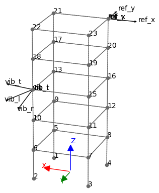
3-D geometry with nodes, structural lines, and channel-DOF arrows — **Geometry view** — nodes (grey dots), structural lines, and channel-DOF arrows showing the oblique measurement directions of each laser head for setup 1. Generated by `ModeShapePlot`.#

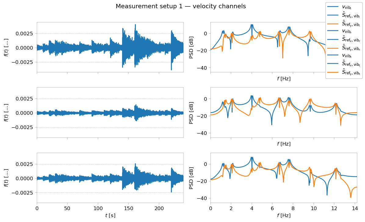
Raw velocity time series (left) and power spectral density (right) — **Measurement signals** — velocity time series (left column) and power spectral densities (right column) for the three vibrometer channels of setup 1 after decimation to ≈ 28 Hz.#

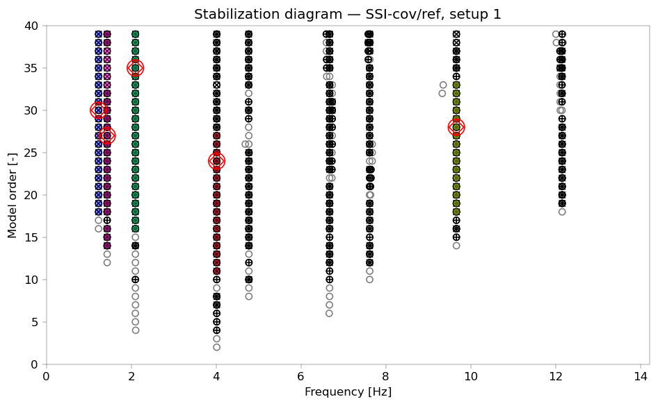
Stabilization diagram with automatically selected poles highlighted — **Stabilization diagram** — all poles computed by SSI-cov/ref up to model order 40 (grey: unstable, black: stable). Red diamonds mark the automatically selected physical modes.#

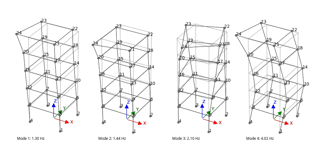
First four mode shapes of the steel-frame test structure side-by-side — **Mode shapes 1–4** (PoGER, all 15 setups merged) — first bending in x, first bending in y, torsion, and second bending, plotted with exaggerated amplitude for clarity.#

The five-step workflow #

Every OMA analysis follows the same five stages:

Step	Class / method	What happens
1	`GeometryProcessor`	Load node coordinates and structural connectivity
2	`PreProcessSignals`	Load the time-series data; assign sampling rate, channel types, and reference channels
3	`correlation()`	Decimate, filter, and compute cross-correlation functions
4	`BRSSICovRef` or other method	Identify modal parameters at multiple model orders
5	`StabilCalc`	Compute the stabilisation diagram and select physical modes

Step 1 – Structural geometry #

from pyOMA.core import GeometryProcessor

geometry_data = GeometryProcessor.load_geometry(
    nodes_file='grid.txt',
    lines_file='lines.txt',               # optional
    parent_childs_file='parent_childs.txt',  # optional
)

GeometryProcessor stores node coordinates and connectivity. It is only required for mode-shape visualisation; you can skip it for a numbers-only analysis.

File formats are described on the Input File Formats page.

To visualise the geometry together with sensor positions before running identification, use ModeShapePlot with only geometry and prep_signals supplied:

from pyOMA.core import ModeShapePlot

geo_plot = ModeShapePlot(geometry_data=geometry_data, prep_signals=prep_signals)
geo_plot.draw_nodes()
geo_plot.draw_lines()
geo_plot.draw_chan_dofs()   # arrows showing sensor measurement directions

Step 2 – Loading measurement signals #

Providing a file loader #

pyOMA is format-agnostic. Before calling init_from_config (or constructing PreProcessSignals directly), you must assign a callable to the class attribute load_measurement_file. It receives the file path and must return an (n_samples, n_channels) NumPy array:

import numpy as np
from pyOMA.core import PreProcessSignals

# NumPy .npy
PreProcessSignals.load_measurement_file = np.load

# Whitespace-separated ASCII
PreProcessSignals.load_measurement_file = lambda f, **kw: np.loadtxt(f)

# Custom binary
PreProcessSignals.load_measurement_file = my_loader

Loading signals directly in Python (recommended for notebooks)#

Construct PreProcessSignals directly from a NumPy array. This is the preferred approach when working interactively — all parameters stay in the notebook and there is no need to maintain separate text files:

import numpy as np
from pyOMA.core import PreProcessSignals

signals = np.load('my_measurement.npy')   # shape (n_samples, n_channels)

prep_signals = PreProcessSignals(
    signals,
    sampling_rate=256,           # Hz
    ref_channels=[2, 3],         # column indices of reference sensors
    accel_channels=[0, 1, 2, 3], # columns measured with accelerometers
    velo_channels=[],            # columns measured with velocimeters
    disp_channels=[],            # columns measured with displacement sensors
    setup_name='my_setup',
)

# Assign channel-DOF information for mode-shape plotting
# (chan, node_name, azimuth_deg, elevation_deg)
prep_signals.chan_dofs = [
    (0, '5',  28.9, -8.7, 'vib_l'),
    (1, '5',  81.0, -7.3, 'vib_r'),
    (2, '24',  0.0, 180.0, 'ref_x'),
    (3, '24', -90.0,  0.0, 'ref_y'),
]

Step 3 – Pre-processing #

Decimation #

decimate_signals() reduces the sampling rate by an integer factor. An anti-aliasing filter is applied automatically before down-sampling. Call it multiple times to achieve large total reduction factors while keeping each step moderate:

prep_signals.decimate_signals(3)   # 256 Hz → 85.3 Hz
prep_signals.decimate_signals(3)   # 85.3 Hz → 28.4 Hz

Filtering #

An optional explicit bandpass filter can be applied before computing correlations if you want to restrict the analysis to a specific frequency band:

prep_signals.filter_signals(lowpass=10.0, highpass=0.1)  # Hz

Correlation functions #

Covariance-driven SSI and PLSCF need the cross-correlation matrix. The Blackman–Tukey method generally gives better frequency resolution:

prep_signals.corr_blackman_tukey(m_lags=200)  # or corr_welch(m_lags=200)

m_lags must satisfy m_lags > num_block_columns + num_block_rows (see Step 4 below).

To inspect signals and correlation functions before running identification, use SignalPlot:

from pyOMA.core import SignalPlot

sig_plot = SignalPlot(prep_signals)

# Time histories and power spectral densities, one row per channel
sig_plot.plot_signals(channels=[0, 1, 2], per_channel_axes=True, psd_scale='db')

# Correlation functions (pass timescale='lags' after calling prep_signals.correlation())
sig_plot.plot_signals(channels=[0, 1, 2], per_channel_axes=True, timescale='lags')

Step 4 – System identification #

All identification methods share the same interface. Pick the class, set the parameters, call the two core methods:

Class	What it needs	Best for
`BRSSICovRef`	Correlations (Step 3)	General ambient vibration, most widely used
`SSIData`	Raw signals	Shorter records; avoids explicit correlation step
`VarSSIRef`	Correlations	When uncertainty (variance) of modal parameters is required
`PLSCF`	Correlations	Frequency-domain alternative to SSI
`ERA`	Impulse response data	Impact-hammer and FRF tests

Example using SSI-cov (recommended — all parameters visible in the notebook):

from pyOMA.core import BRSSICovRef

modal_data = BRSSICovRef(prep_signals)
modal_data.build_toeplitz_cov(num_block_columns=100)  # must be < m_lags
modal_data.compute_modal_params(max_model_order=40)

Example using SSI-data directly:

from pyOMA.core import SSIData

ssi = SSIData(prep_signals)
ssi.build_block_hankel(num_block_rows=100)
ssi.compute_modal_params(max_model_order=40)

Example using PLSCF directly:

from pyOMA.core import PLSCF

plscf = PLSCF(prep_signals)
plscf.build_half_spectra(
    nperseg=200,            # correlation lag length (same as m_lags)
    begin_frequency=0.0,   # Hz
    end_frequency=12.0,    # Hz
)
plscf.compute_modal_params(max_model_order=40)

Key parameters #

num_block_columns / num_block_rows: Number of block rows/columns in the block-Toeplitz or Hankel matrix. Higher values capture longer time correlations but increase computation time. Typical range: 50–200. Must satisfy num_block_columns + num_block_rows < m_lags.
max_model_order: The algorithm estimates modal parameters at every order from 1 up to this value. Stable physical modes appear across many orders. Typical range: 20–100. Setting it to 2 × expected_number_of_modes is a safe starting point.

Step 5 – Stabilisation diagram #

from pyOMA.core import StabilCluster, StabilPlot

stabil_calc = StabilCluster(modal_data)

# Compute hard-criteria masks
stabil_calc.calculate_stabilization_masks(
    d_range=(0, 0.10),   # damping 0–10 %
    df_max=0.01,          # max relative frequency change between orders
    dd_max=0.05,          # max relative damping change between orders
    dmac_max=0.05,        # max MAC change between orders
)

# Static plot
stabil_plot = StabilPlot(stabil_calc)
stabil_plot.plot()

# Automated mode selection
stabil_calc.automatic_clearing()
stabil_calc.automatic_classification()

# Export results to a tab-separated text file
stabil_calc.export_results('modes.txt')

Pole stability criteria #

d_range: Absolute damping ratio limits (min, max).
df_max, dd_max: Maximum relative change in frequency / damping between consecutive model orders. A pole that shifts by more than df_max × 100 % between order n and n+1 is considered new/unstable.
dmac_max: Maximum MAC difference between mode shapes at consecutive orders. Ensures that the shape is consistent and not just a numerical artefact.

Choosing thresholds #

There is no universal set of thresholds. As a starting point:

For lightly damped civil structures: df_max=0.01, dd_max=0.05, dmac_max=0.05, d_range=(0, 0.05).
For more heavily damped mechanical systems: loosen d_range and dd_max accordingly.
Always inspect the raw stabilisation diagram visually before accepting automatically selected modes.

Example scripts and notebooks #

Four ready-to-run examples are included in the scripts/ directory. The first three are each available as a plain Python script (requires pip install "pyOMA[gui]") and as an interactive Jupyter notebook (requires pip install "pyOMA[jupyter]"):

Scenario	Script	Notebook
Single setup	`scripts/single_setup_analysis.py`	pyOMA – Single-Setup Operational Modal Analysis
Multi-setup — PoSER (post-identification merging)	`scripts/multi_setup_analysis.py`	pyOMA – Multi-Setup OMA with PoSER merging
Multi-setup — PoGER (pre-identification merging)	`scripts/multi_setup_analysis_poger.py`	pyOMA – Multi-Setup OMA with PoGER merging
Single setup, GUI-only (every step done interactively)	`scripts/single_setup_analysis_gui_only.py`	— (interactive only, see GUI Usage)

The PoSER workflow runs SSI independently on each measurement setup and then merges the estimated modal parameters using MergePoSER. The PoGER workflow stacks correlation functions from all setups into a joint Hankel matrix before a single SSI run, yielding global frequencies, damping ratios, and re-scaled mode shapes directly via PogerSSICovRef.

The bundled example data originates from ambient vibration measurements on a steel-frame test structure using a Polytec PSV 400-3D three-head scanning laser vibrometer, with each laser head measuring in an oblique (skewed) direction relative to the structure. A detailed description of the test structure, the 3D-SLDV measurement principle, and the 15-setup scan arrangement is given on the Example data: steel frame with 3D scanning laser vibrometer page.