GUI Usage#

This page walks through every window of pyOMA’s desktop GUI, in the order you would normally open them. Screenshots are generated from the bundled steel-frame example data (see Example data: steel frame with 3D scanning laser vibrometer) by scripts/generate_gui_screenshots.py — run that script and commit the result whenever a GUI window’s layout changes, so these images never go stale (see GUI Development for the full workflow).

Overview #

pyOMA has two interactive frontends:

PyQt6 desktop GUI (this page) — standalone windows, installed with pip install -e ".[gui]". Covers the whole workflow: geometry editing, signal pre-processing, system identification, stabilisation, and mode-shape visualisation.
Jupyter/ipywidgets GUI — inline notebook widgets, installed with pip install -e ".[jupyter]". Covers stabilisation and mode-shape visualisation only. See Jupyter/ipywidgets alternative below.

Both wrap the same underlying classes described in Getting Started; neither is required to use pyOMA — everything is also directly scriptable, as that page shows.

Closing any desktop-GUI window with unsaved changes offers to Save, Continue (close without saving), or Cancel.

Quickest start: the `pyoma` launcher #

Once installed with pip install -e ".[gui]", pyoma opens MultiSetupGUI with nothing pre-loaded - no example data, no script, no config files required:

pyoma

From there:

Pick Single Setup mode (top mode selector) for one measurement, or PoSER/PoGER for multiple - see 6. Single- and multi-setup analysis — MultiSetupGUI below for what each mode does.
Click Add Setup, then in the new tab click Pre-process Signals… - this is the tab’s entry point, opening PreProcessSignalsGUI empty. Loading itself happens from inside that window’s File menu, not the tab:
- File → Load Config… prompts for a config file, then a measurement file, and loads them via init_from_config() - the same entry point every scripted workflow on this page uses. A bare .npy measurement file loads out of the box with no setup required (a warning is logged noting that channel headers/units/start time are synthesized); for any other measurement-file format, assign a custom PreProcessSignals.load_measurement_file first - see scripts/converters/ for examples.
- File → Import Signals… loads a bare .npy array (prompts for the sampling rate) or an already-packaged .npz session directly, with no config file at all.
- File → Load State… resumes a session saved via File → Save State….
Closing that window hands whatever ended up loaded back to the tab.
Continue through pre-processing, identification, and (in Single Setup / PoSER mode) pole selection from inside that same tab - each button in the tab’s Pipeline box opens the next window in sequence.
Once ready, the Continue/Merge Setups button (label depends on mode) takes you to the merged (or, in Single Setup mode, single) mode shapes.

This is the same underlying pipeline as every workflow described below on this page - it’s the entry point with the fewest prerequisites, not a different feature set. The rest of this page documents each window in more depth, and the _gui_only scripts remain useful as ready-to-run demonstrations against the bundled example data.

Recommended way to explore: single_setup_analysis_gui_only.py #

The quickest way to see every window below, interactively, against the bundled example data:

python scripts/single_setup_analysis_gui_only.py

Unlike scripts/single_setup_analysis.py (which pre-computes decimation, correlation, and identification parameters in code and only optionally opens a GUI afterwards, via its SHOW_*_GUI flags), the _gui_only variant makes every one of those decisions interactively — you pick the decimation factor, correlation/PSD parameters, identification method, and stabilisation thresholds inside the GUIs themselves. What remains scripted is only what has no GUI equivalent yet: loading the initial measurement and wiring one GUI’s output into the next one’s input.

scripts/multi_setup_analysis.py (PoSER) and scripts/multi_setup_analysis_poger.py (PoGER) offer the same SHOW_GEOMETRY_GUI/SHOW_PREPROCESS_GUI flags (plus SHOW_MODAL_GUI for PoSER, which identifies each setup individually) to open GeometryProcessorGUI, PreProcessSignalsGUI, and ModalAnalysisGUI for interactive inspection as the per-setup loop runs, alongside their existing MANUAL_POLE_SELECTION/ SHOW_MODE_SHAPES flags for the stabilisation diagram and merged mode shapes. PoGER has no per-setup modal-ID GUI step, since it identifies all setups jointly after pooling rather than per setup.

For a fully interactive multi-setup workflow, run scripts/multi_setup_analysis_gui_only.py, the multi-setup counterpart of single_setup_analysis_gui_only.py above. It opens MultiSetupGUI directly instead of the scripted loop: PoSER/PoGER mode, geometry, adding setups (each one loaded via its tab’s “Pre-process Signals…” → File → Load Config…), and every downstream step (pre-processing, identification, stabilisation, PoGER’s block-column/model-order settings, and merging) are all driven from that one window.

1. Geometry — GeometryProcessorGUI #

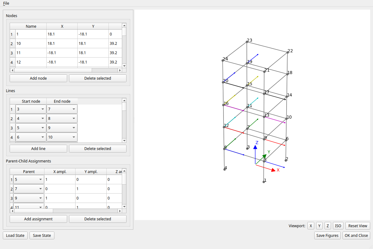
Geometry editor showing node, line, and parent-child tables next to a 3-D structure preview — **Geometry editor** — add/edit/delete nodes, structural lines, and parent-child (oblique-DOF decomposition) assignments, with a live 3-D preview. Wraps `GeometryProcessor`.#

Launch standalone with start_geometry_processor_gui(). This step is optional — skip it if you only need numerical results, not mode-shape visualisation.

2. Signal pre-processing — PreProcessSignalsGUI #

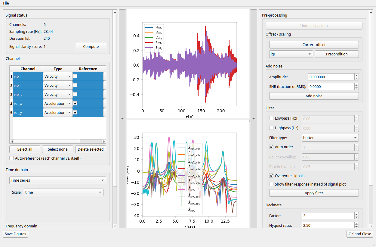
Pre-processing window showing the channel table, time/PSD plots, and processing controls — **Signal pre-processing** — channel table (type, reference flag, rename, delete), time-series/PSD/correlation plots, and controls for offset correction, filtering, and decimation. Wraps `PreProcessSignals` and `SignalPlot`.#

Launch standalone with start_preprocess_gui().

This window can also be opened with no data at all (start_preprocess_gui(), no arguments) - every control except the File menu stays disabled until a signal is loaded, via one of:

File → Load Config… - prompts for a config file, then a measurement file, and loads them via init_from_config().
File → Import Signals… - a bare .npy array (prompts for the sampling rate) or an already-packaged .npz session, with no config file needed.
File → Load State… - resumes a session saved via File → Save State….

File → Save Config… writes a config file that init_from_config() can read back - useful for turning an interactively-built setup into a reusable, scriptable one - and File → Load/Save Channel DOFs… bulk round-trip the channel-DOF assignments made via the “Add DOF” button below, in the tab-separated format documented in Input File Formats.

Channel-DOF assignment — ChanDofEditorGUI #

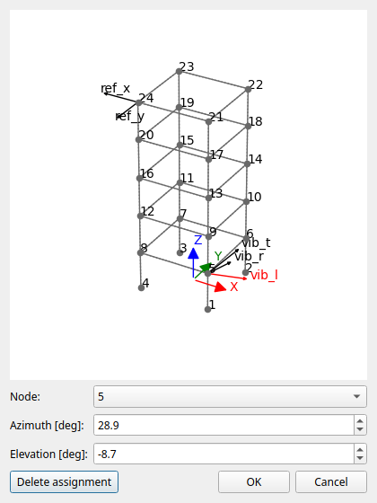
Dialog for assigning a channel's measurement node, azimuth, and elevation — **Channel-DOF editor** — opened via the channel table’s “Add DOF” button (or by double-clicking an assigned channel); picks the node a channel measures at and its azimuth/elevation, with a live 3-D preview of the resulting sensor direction.#

3. System identification — ModalAnalysisGUI #

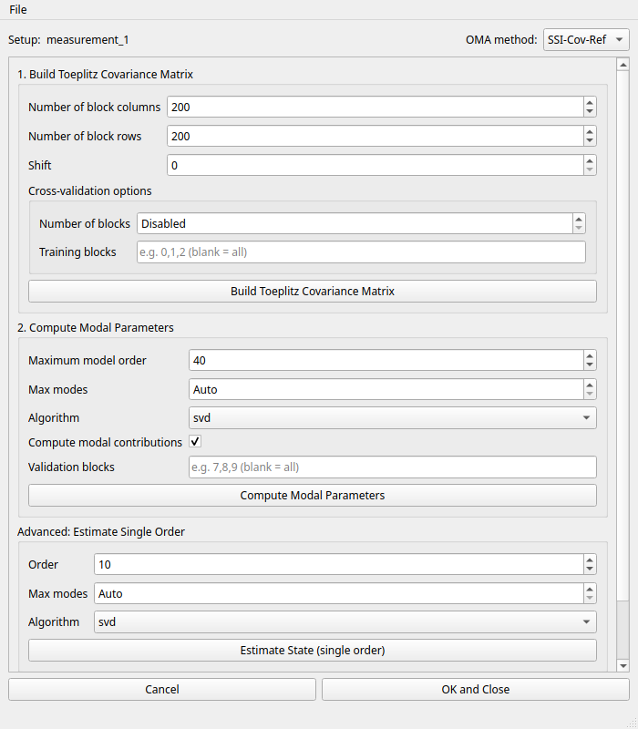
Modal analysis window on its SSI-Cov-Ref page, showing build/compute controls and computed status — **System identification** — a method selector and a build/compute page per method, applied to the same pre-processed signals. Shown here on the SSI-Cov-Ref page after both build steps have run. Launch standalone with `start_modal_analysis_gui()`.#

Every method page follows the same pattern: fill in the parameters for each step, click the step’s button, then click “Save State…”/”Load State…” to persist or restore the underlying object. See Getting Started’s Step-4 table for when to choose each method. The other four pages — SSI-Data (SSIData family: SSI-Data, SSI-Data/MC, SSI-Data/CV, picked via a variant combo box), Var-SSI-Ref (VarSSIRef, an extra “prepare sensitivities” step for uncertainty quantification), pLSCF (PLSCF), and PRCE (PRCE, requires at least 2 reference channels) — share this same two-or-more-step build/compute layout with method-specific parameters.

4. Stabilisation diagram — StabilGUI #

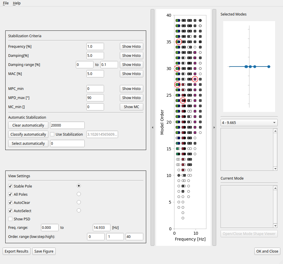
Stabilization diagram with adjustable criteria, pole classification, and view settings — **Stabilisation diagram** — adjustable stabilisation criteria, automatic pole clearing/classification/selection, and a mode-value inspector. Wraps `StabilPlot` and `StabilCluster`. Launch standalone with `start_stabil_gui()`.#

Clicking a pole (or stepping through the mode selector once modes are selected) updates the display of the complex-plane.

5. Mode-shape animation — ModeShapeGUI #

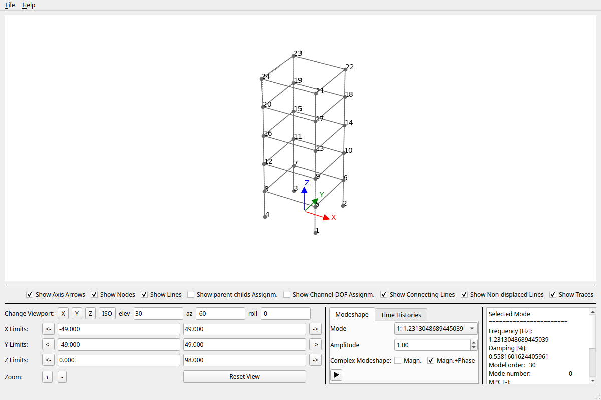
Mode-shape viewer with a 3-D animated view and per-mode information panel — **Mode-shape viewer** — animated 3-D mode shapes with amplitude scaling, node/line/trace visibility toggles, and per-mode frequency/damping/order information. Wraps `ModeShapePlot`. Launch standalone with `start_msh_gui()`.#

This same viewer is also embedded live inside StabilGUI (pass msh_plot to start_stabil_gui) so the mode shape updates immediately as you select poles — the screenshot above shows it standalone, with its full control panel.

6. Single- and multi-setup analysis — MultiSetupGUI #

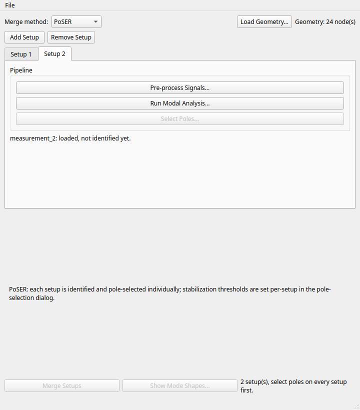
Multi-setup GUI showing one tab per measurement setup, a PoSER/PoGER mode switch, and merge controls — **Multi-setup merging** — one tab per measurement setup (each launching the windows above to pre-process, identify, and pole-select that setup), a PoSER/PoGER mode switch, and a merge step producing the global mode shapes. Shown here with two setups loaded (PoSER mode). Wraps `MergePoSER` (PoSER) or `PogerSSICovRef` (PoGER). Launch standalone with `start_multi_setup_gui()`.#

A third mode - Single Setup - handles the one-measurement case in the same window: adding a second tab is disabled, there is nothing to merge, and the button that says “Merge” in PoSER/PoGER mode instead reads “Continue” and takes the one tab’s own modal identification and pole-selection results straight to the mode-shape viewer. This makes MultiSetupGUI (via the pyoma launcher, or start_multi_setup_gui()) the recommended starting point regardless of how many setups you have - see “Quickest start” above.

Each setup’s tab is just a Pipeline box: “Pre-process Signals…” is the entry point - loading itself happens inside that window’s File menu, see “Quickest start” above - followed by, in PoSER/Single Setup mode, “Run Modal Analysis…” and “Select Poles…” (identification and pole-selection happen per setup, then merge). In PoGER mode those two buttons are hidden, since PoGER identifies and pole-selects all pooled setups jointly, once, after merging - which needs each setup’s correlation function already computed (via “Pre-process Signals…” → the Correlation time-domain diagram, or scripted), since merging pools the correlation matrices directly rather than recomputing them. Geometry is loaded once via “Load Geometry…” and shared across every setup’s dialogs. Run python scripts/multi_setup_analysis_gui_only.py for the quickest way to try this interactively.

Jupyter/ipywidgets alternative #

For notebook-based work, pyOMA.GUI.JupyterGUI provides inline equivalents of the stabilisation diagram and mode-shape viewer, plus a config file editor:

from IPython.display import display
from pyOMA.GUI.JupyterGUI import StabilGUIWeb, PlotMSHWeb, ConfigGUIWeb

widget, cursor = StabilGUIWeb(stabil_plot)
display(widget)

display(PlotMSHWeb(mode_shape_plot))

See Getting Started for installation (pip install -e ".[jupyter]") and the worked example notebooks under Examples.