Multi-Setup PoGER Analysis of a Guyed Mast#

This page describes how pyOMA has been applied to an ambient-vibration measurement campaign on a guyed steel-tube telecommunication mast, using the covariance-driven, reference-based Stochastic Subspace Identification method (SSI-cov-ref) merged across several measurement setups with the PoGER (Post Global Estimation Re-scaling) strategy. Guyed masts are a challenging case for operational modal analysis: the three-fold rotational symmetry of a typical guying arrangement produces closely spaced pairs of bending modes in near-orthogonal directions, and the strongly nonlinear, temperature- and amplitude-dependent stiffness of the guy cables raises the question of whether a linear, time-invariant identification method can meaningfully describe the structure’s dynamics at all.

Structure and instrumentation#

The mast is a steel tube of tubular cross-section, approximately 197 m tall, stabilized by guy cables arranged in three lanes at 120° azimuthal spacing and attached at four stay levels along the height. Ambient vibrations were measured with piezoelectric accelerometers (PCB 393B31) recording two horizontal, orthogonal directions at 14 measurement points along the mast, sampled at 128 Hz for 30 minutes per setup. Two sensor pairs at fixed reference positions remained in place throughout the campaign; four additional roving sensor pairs were moved between three measurement setups to cover the full height of the mast.

Measurement campaign#

The three roving setups (referred to here as Setup 1, 2, and 3) together cover 14 measurement points at 2 orthogonal horizontal directions each. A second campaign variant additionally instrumented the guy cables themselves at their four stay levels, adding four more setups analyzed the same way — this “cables” variant is not detailed further here, but uses an identical pyOMA workflow.

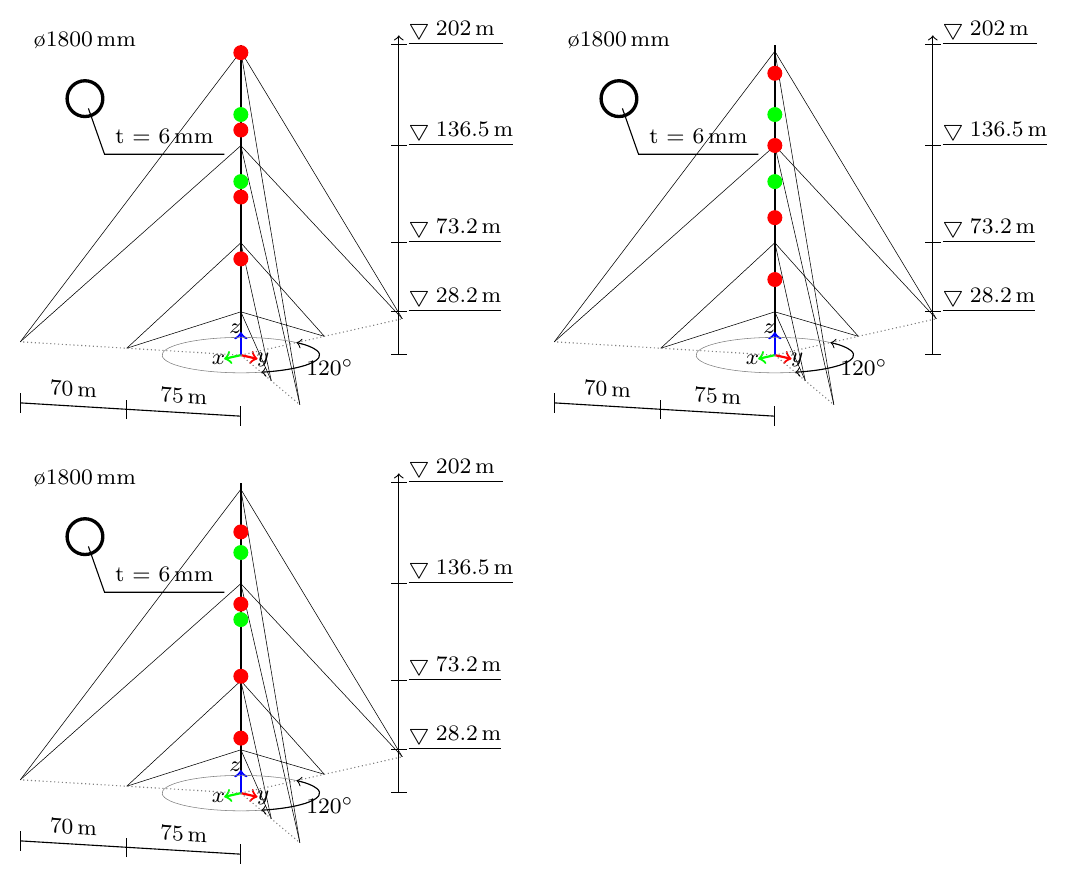
Mast elevation showing sensor positions for the three setups — Mast elevation drawing, cycling through the three measurement setups. Green markers are the two fixed reference sensor pairs; red markers are the four roving sensor pairs, repositioned between setups to cover the full mast height.#

Because modal density was very high below approximately 1.5 Hz, the frequency range was split and processed in two separate passes: a low- frequency band (0.1–1.5 Hz) and a high-frequency band (1.5–8 Hz), each with its own bandpass filter, decimation factor, and correlation-function lag count, sized to resolve that band’s mode count with an adequate number of block rows in the SSI Hankel matrix.

pyOMA integration#

The identification is implemented with pyOMA’s PogerSSICovRef, which merges the setups before the state-space identification step rather than merging separately identified mode shapes afterwards (the alternative PoSER — Post Separate Estimation Re-scaling — approach implemented in MergePoSER). PoGER was chosen here to reduce the manual identification effort across the many setups of the full campaign.

1. Geometry and per-setup preprocessing

import numpy as np
from pyOMA.core.PreProcessingTools import GeometryProcessor, PreProcessSignals
from pyOMA.core.SSICovRef import PogerSSICovRef

geometry = GeometryProcessor.load_geometry(nodes_file, lines_file)

# raw measurements are plain ASCII column files
PreProcessSignals.load_measurement_file = np.loadtxt

poger = PogerSSICovRef()
for conf_file, meas_file, chan_dofs_file in setups:
    prep = PreProcessSignals.init_from_config(
        conf_file, meas_file, chan_dofs_file,
    )
    prep.filter_signals(highpass=0.1, lowpass=1.5)
    prep.decimate_signals(5)
    prep.decimate_signals(5)          # combined decimation factor 25 -> ~5.1 Hz
    prep.correlation(m_lags=422)       # >= 2 * num_block_rows + 2
    poger.add_setup(prep)

Each setup’s PreProcessSignals object is built via init_from_config(), which reads the sampling rate, reference/roving channel indices, and sensor axis assignment from a plain-text per-setup configuration file, keeping per-setup metadata out of the analysis code.

2. PoGER merging and identification

poger.pair_channels()
poger.build_merged_subspace_matrix(num_block_columns=210)
poger.compute_modal_params(max_model_order=200)

pair_channels() matches degrees of freedom that are common to all setups (the fixed reference sensor pairs) and uses them to rescale each setup’s partial mode shapes onto a single common reference by joint least squares — no per-setup single-setup identification is needed before merging.

3. Stabilization

from pyOMA.core.StabilDiagram import StabilCluster

stabil = StabilCluster(poger)
stabil.calculate_soft_critera_matrices()
stabil.calculate_stabilization_masks(
    d_range=(0.01, 1), mpc_min=0.5, mpd_max=30,
    df_max=0.001, dd_max=0.1, dmac_max=0.001,
)
stabil.automatic_selection()

The stabilization thresholds above are the ones used for this dataset; automatic_selection() performs an unsupervised clearing/clustering/selection pass, though the original study selected modes interactively via the stabilization-diagram GUI instead.

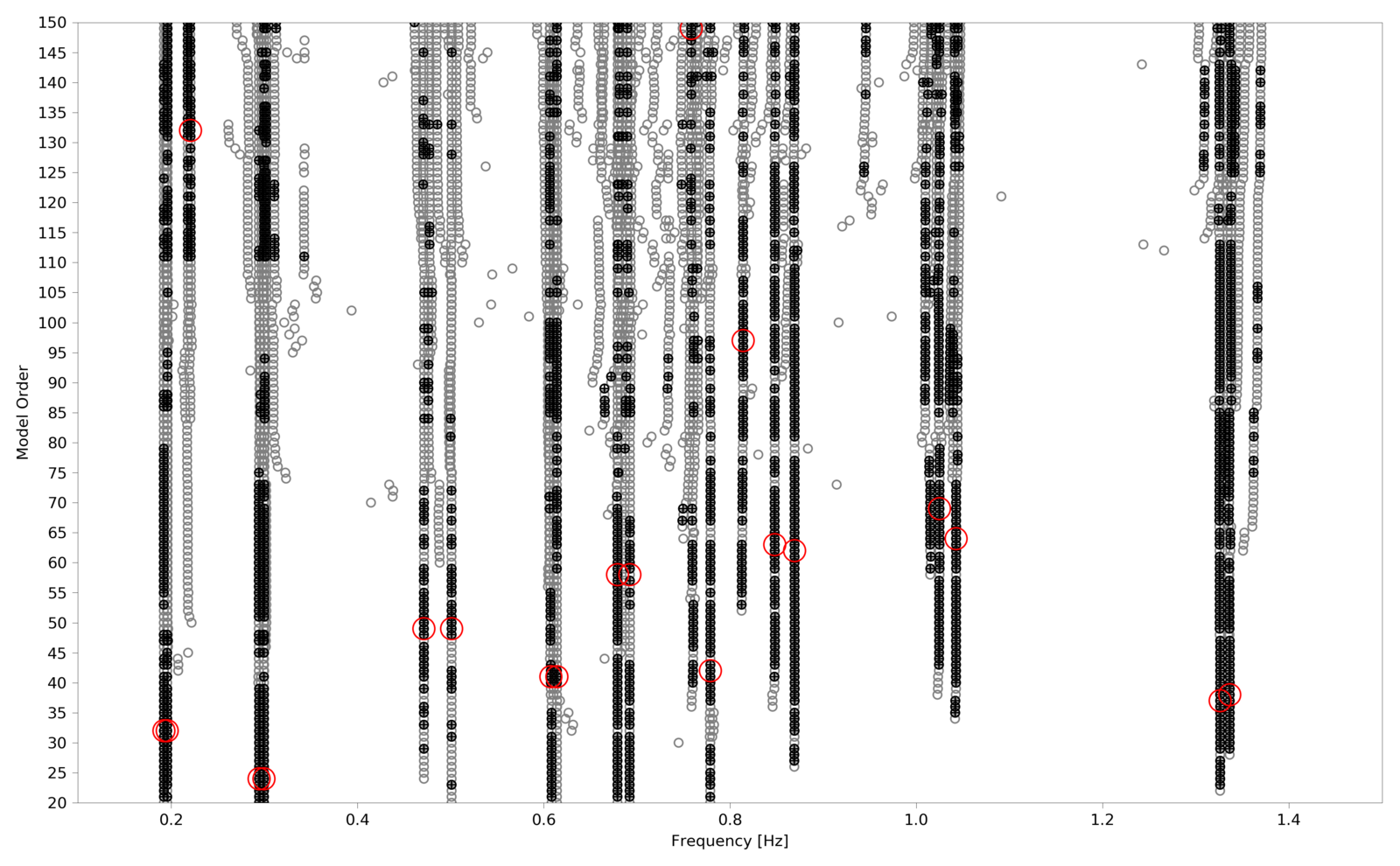
Stabilization diagram, low-frequency band — Stabilization diagram for the low-frequency band (0.1–1.5 Hz). Gray circles are identified poles at each model order; black-filled circles passed the stability criteria; red circles mark the poles selected as physical modes.#

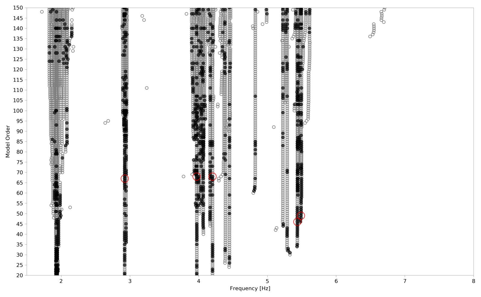
Stabilization diagram, high-frequency band — Stabilization diagram for the high-frequency band (1.5–8 Hz), same convention as above.#

4. Mode-shape visualization

from pyOMA.core.PlotMSH import ModeShapePlot

mode_shape_plot = ModeShapePlot(
    geometry_data=geometry, modal_data=poger, stabil_calc=stabil,
    prep_signals=poger.prep_signals, amplitude=10,
)
mode_shape_plot.save_plot('mode_shape.png')

Results#

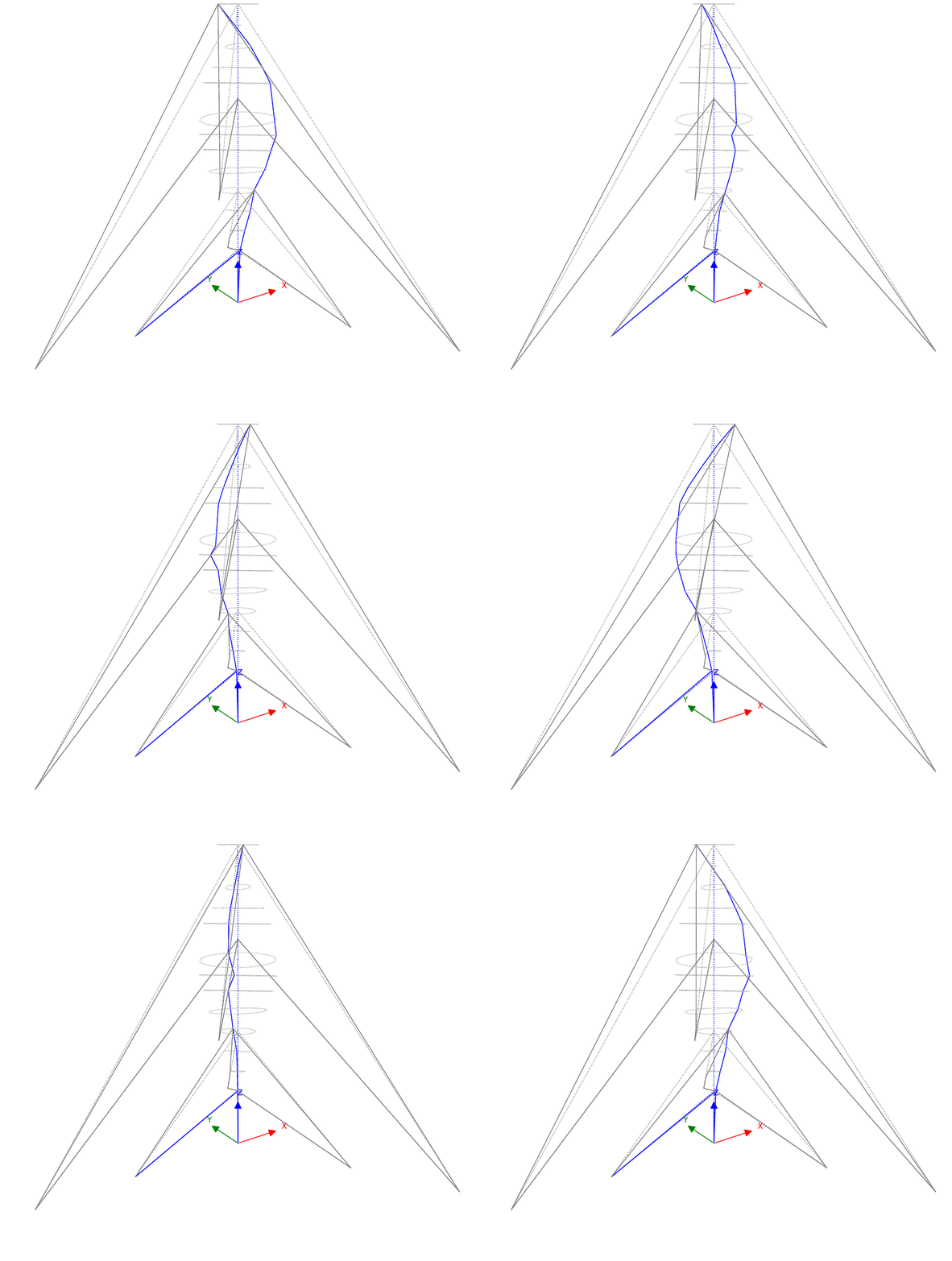
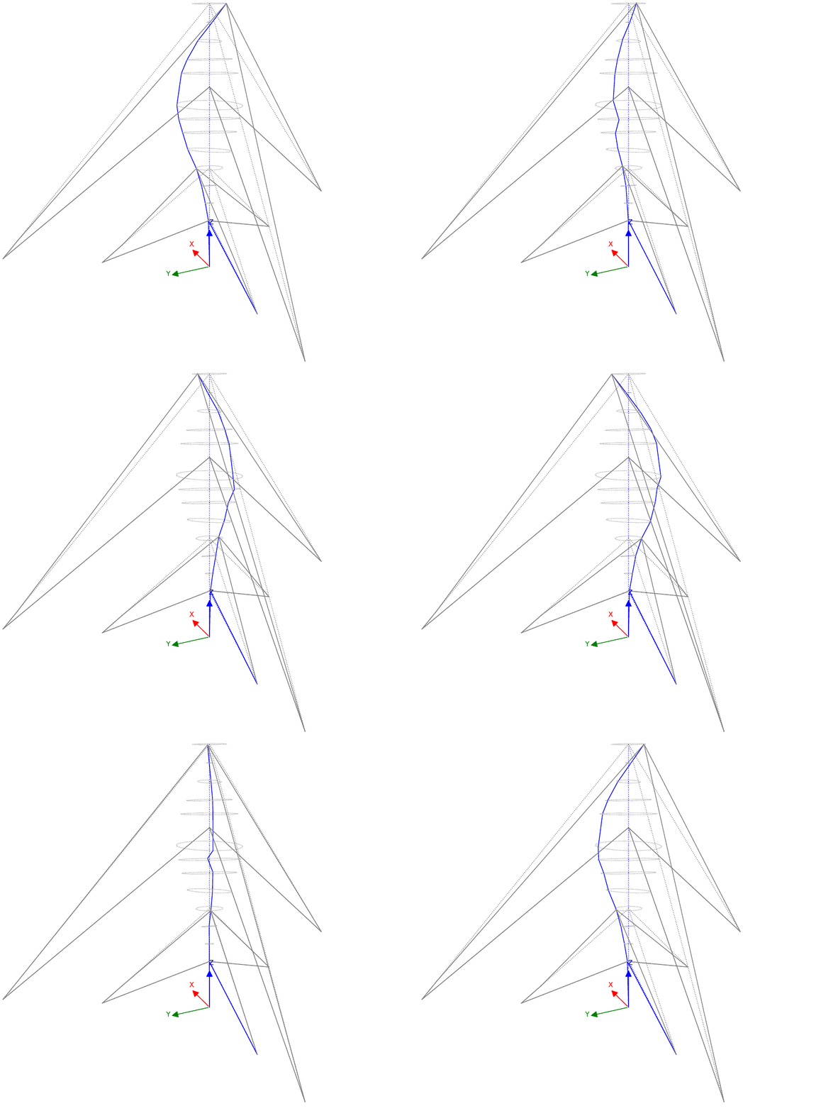
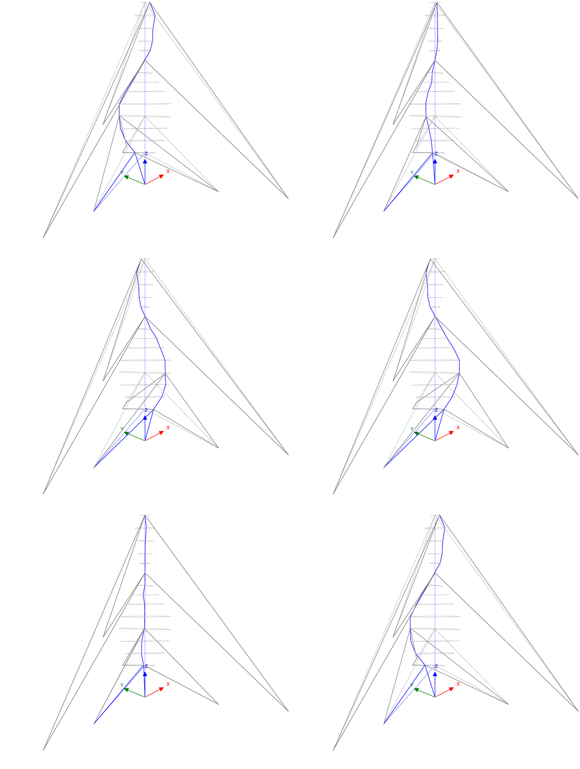
30 modes were identified up to approximately 5.5 Hz. As expected from the mast’s three-fold rotationally symmetric guying arrangement, modes appear in closely spaced pairs vibrating in near-orthogonal directions — visible below as pairs of near-identical frequencies with principal directions roughly 90° apart. In addition to the frequency and damping ratio estimated directly by pyOMA, the study computed a principal vibration direction (α) for each mode — the azimuth of the major axis of the (generally elliptical) horizontal displacement orbit, obtained via a custom orthogonal least-squares fit of the two horizontal mode-shape components. This direction analysis is domain-specific post-processing beyond pyOMA’s built-in API.

The animations below show the identified deformation of the first six mode pairs (modes 1–6 and 13–18), each looping over one oscillation cycle:

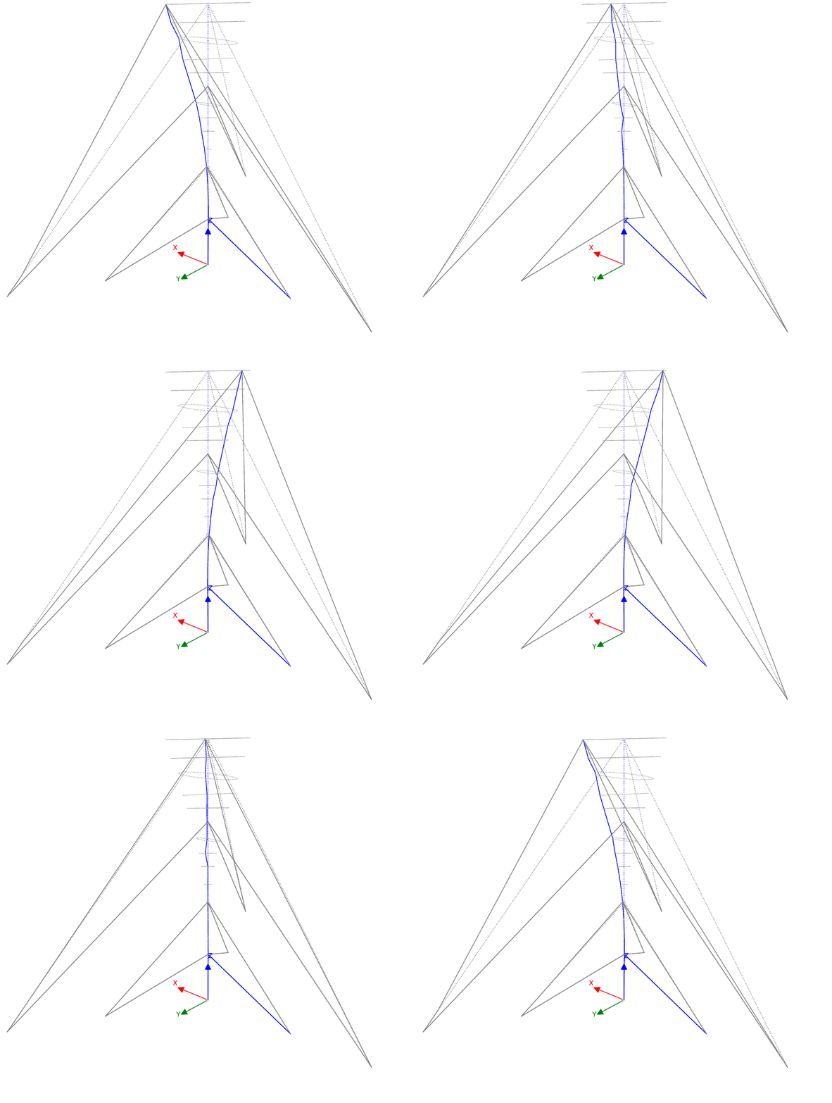
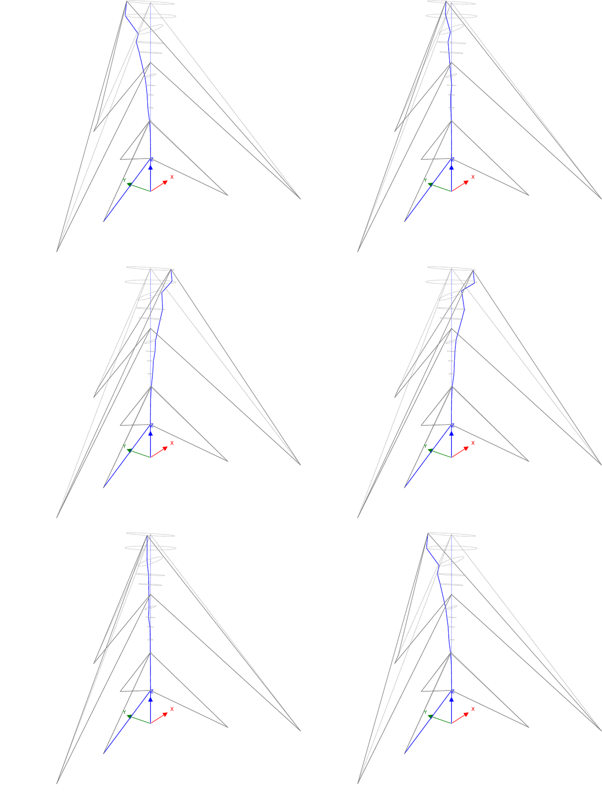
Mode 1 — f = 0.196 Hz, ζ = 0.47 %, α = 41°	Mode 2 — f = 0.192 Hz, ζ = 0.48 %, α = 117°
Mode 3 — f = 0.295 Hz, ζ = 0.34 %, α = 151°	Mode 4 — f = 0.300 Hz, ζ = 0.27 %, α = 64°
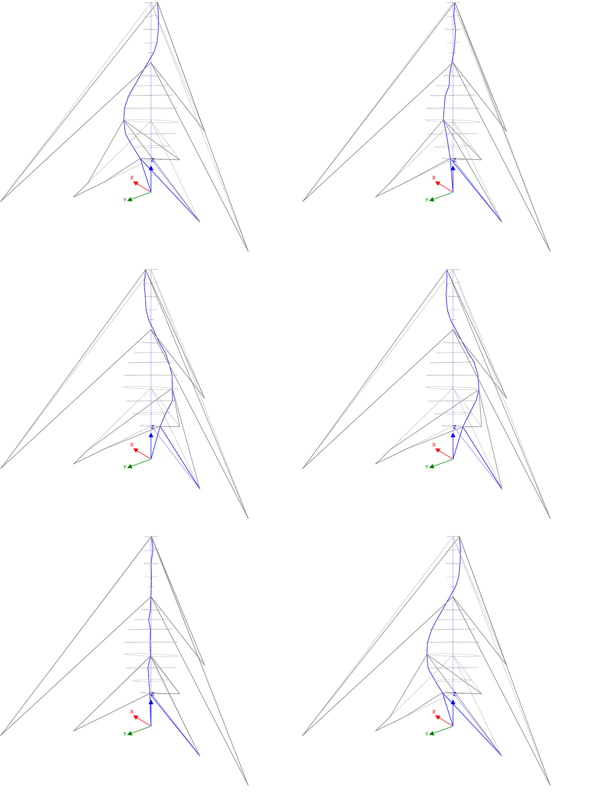
Mode 5 — f = 0.471 Hz, ζ = 0.62 %, α = 133°	Mode 6 — f = 0.501 Hz, ζ = 0.37 %, α = 52°
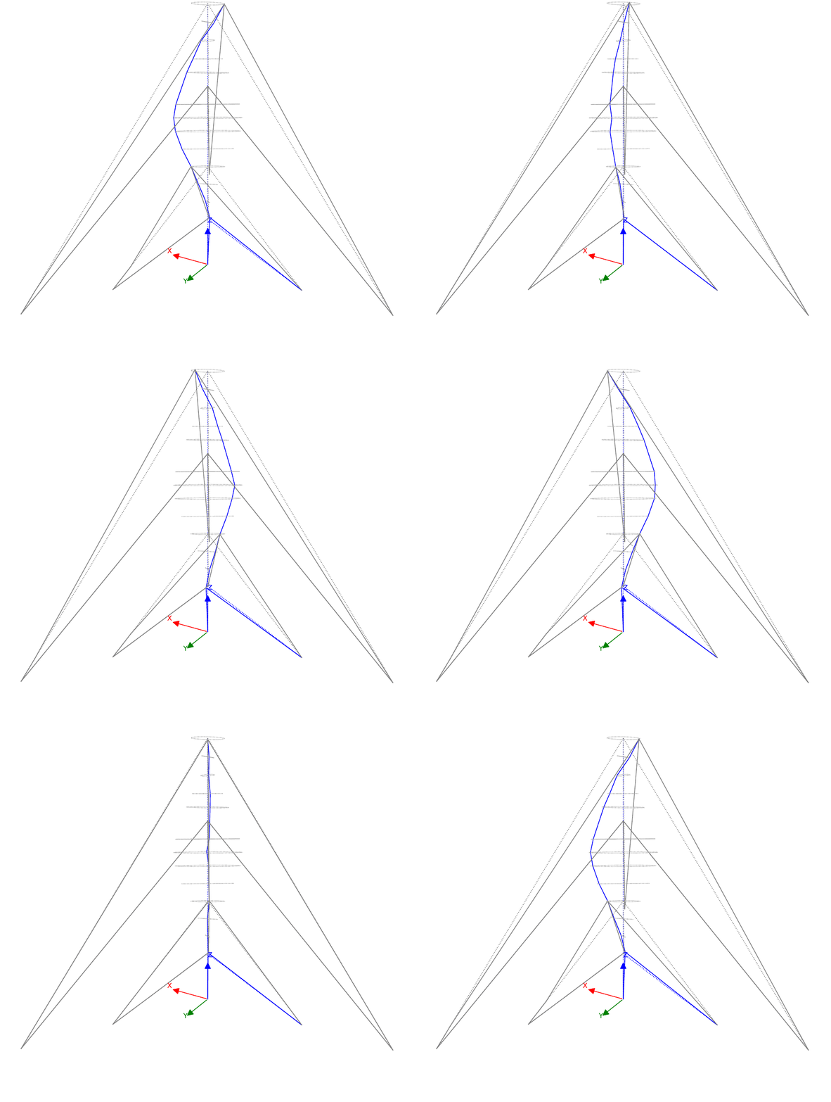
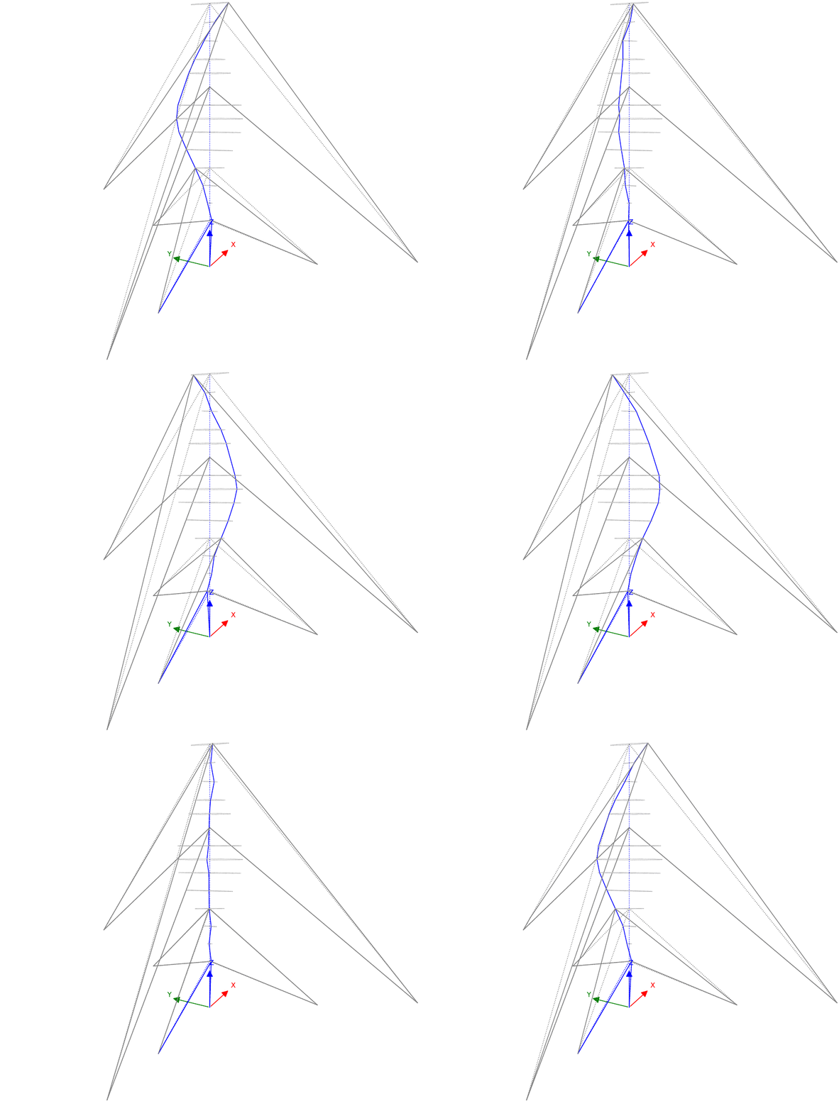
Mode 13 — f = 0.848 Hz, ζ = 0.50 %, α = 31°	Mode 14 — f = 0.869 Hz, ζ = 0.22 %, α = 116°
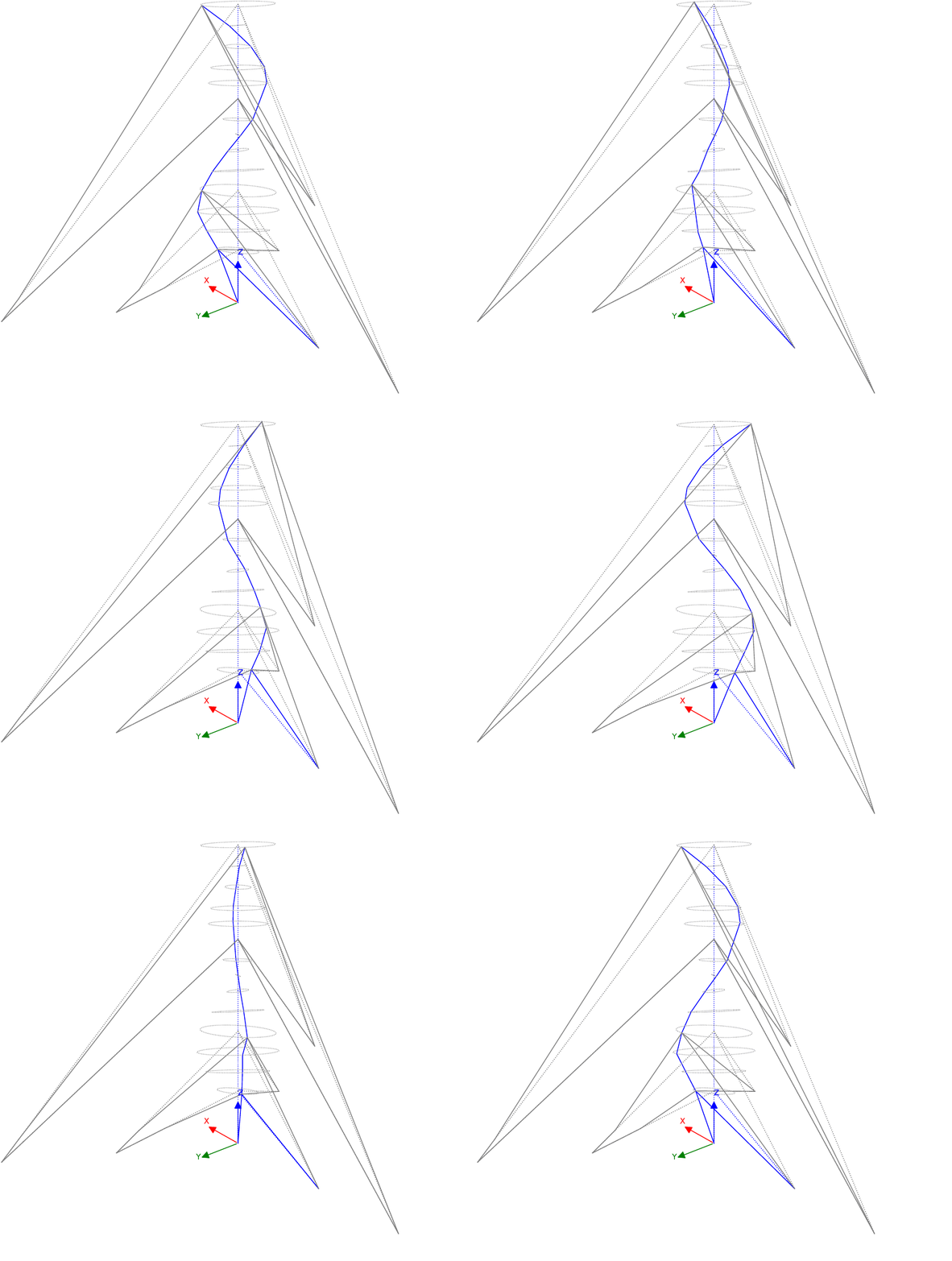
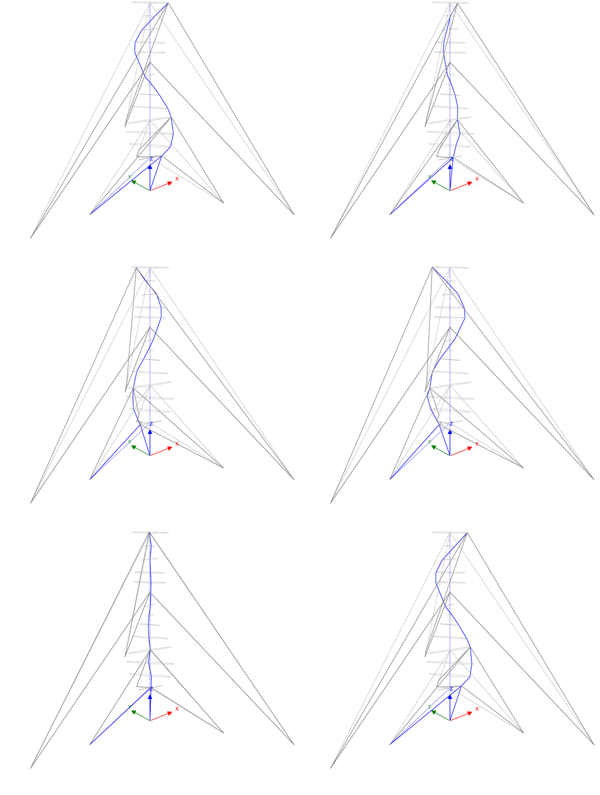
Mode 15 — f = 1.024 Hz, ζ = 0.47 %, α = 46°	Mode 16 — f = 1.043 Hz, ζ = 0.25 %, α = 137°
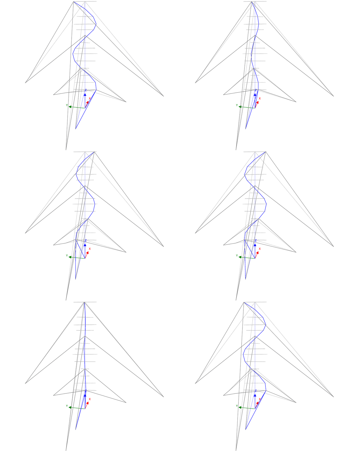
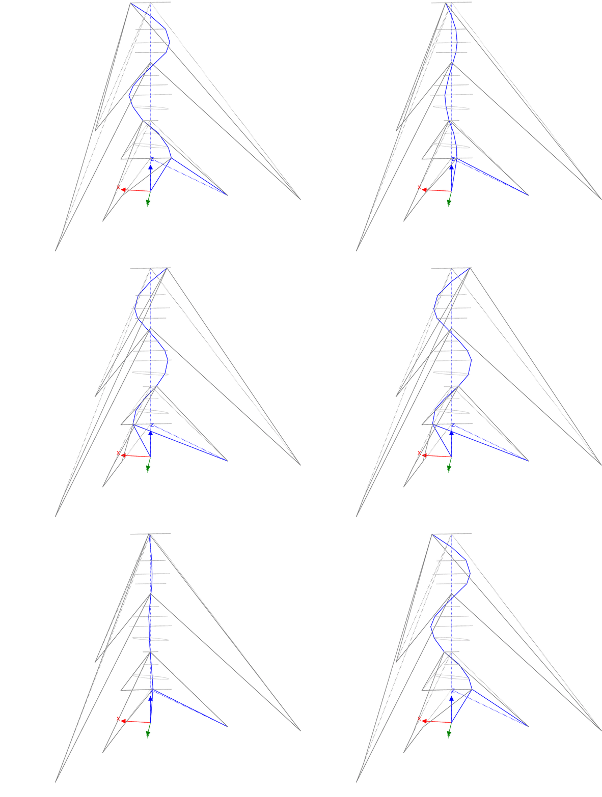
Mode 17 — f = 1.326 Hz, ζ = 0.29 %, α = 102°	Mode 18 — f = 1.336 Hz, ζ = 0.23 %, α = 5°

The complete set of 30 identified modes is listed below.

Identified modal parameters#
Mode	f [Hz]	ζ [%]	α [°]
1	0.196	0.466	41.13
2	0.192	0.479	117.14
3	0.295	0.338	151.25
4	0.300	0.269	63.79
5	0.471	0.615	132.52
6	0.501	0.365	52.19
7	0.609	0.189	24.63
8	0.614	0.207	106.23
9	0.679	0.185	15.72
10	0.692	0.310	103.23
11	0.779	0.426	87.16
12	0.814	0.285	159.03
13	0.848	0.495	31.24
14	0.869	0.224	116.13
15	1.024	0.468	45.90
16	1.043	0.253	137.08
17	1.326	0.291	102.40
18	1.336	0.227	4.95
19	1.930	0.307	181.20
20	1.937	0.111	93.56
21	2.924	0.346	130.87
22	2.942	0.495	35.56
23	3.972	0.550	54.87
24	4.201	0.276	55.87
25	3.973	0.553	52.35
26	4.200	0.195	1.41
27	4.390	0.385	114.28
28	4.449	0.267	33.29
29	5.439	0.494	69.28
30	5.494	0.673	152.53

References#

[BAUSTATIK2020]

Zabel, V., Marwitz, S., and Habtemariam, A. (2020). “Bestimmung von modalen Parametern seilabgespannter Rohrmasten.” Baustatik-Baupraxis.