Continuous Structural Health Monitoring#

This page describes how pyOMA has been deployed in a long-term continuous Structural Health Monitoring (SHM) campaign for an approximately 190 m tall telecommunication tower that has been in operation since 2015. Acceleration (100 Hz) and fibre Bragg grating (FBG) strain data (20 Hz), together with wind and temperature measurements, are transmitted daily from the tower to a central server, where a fully automated pipeline identifies five bending mode pairs in the frequency range 0.35–3.5 Hz and stores the results in a time-indexed database.

Find a comprehensive documentation of the pyOMA-Monitoring project at pyOMA-monitoring docs.

Structure and instrumentation#

The tower consists of three structural sections: a tapered prestressed concrete shaft at the base, a tubular steel section in the middle, and a glass-fibre reinforced plastic (GRP) cylinder at the top. The tower’s slender shape makes it susceptible to wind-induced vibrations. A tuned mass damper (TMD) — a steel–concrete ring of approximately 1000 kg hanging on short pendulum rods — is installed at the top to attenuate vibrations in the frequency range 1.5–2.5 Hz.

The monitoring system was installed in three stages over several years. Piezoelectric accelerometers measuring horizontal vibrations in two orthogonal directions are installed in pairs at five height levels between approximately 100 m and 190 m. Two ultrasonic anemometers (at the top and at mid-height) and five PT100 temperature sensors record environmental conditions. In a later expansion stage, FBG strain rosettes were added at the steel–concrete transition zone to capture local strains independently of the accelerometer network. All analog signals are digitised at distributed stations and transmitted via fibre-optic link to a controller at ground level, from which data are downloaded to a processing server once per day.

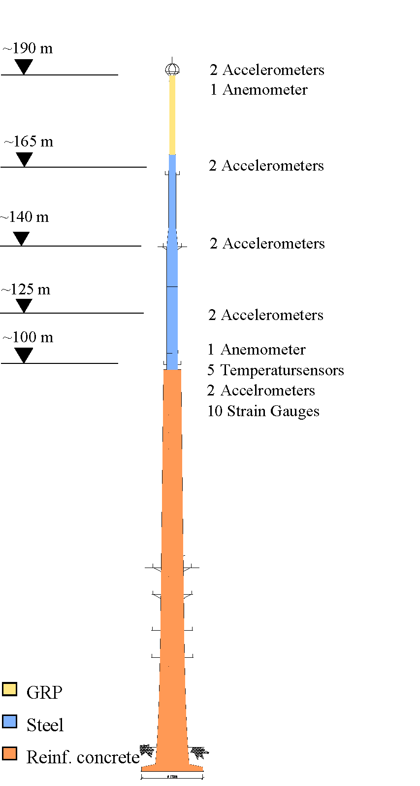
Sensor layout of the telecommunication tower. Accelerometer pairs are installed at five height levels (≈100–190 m); an anemometer and temperature sensors are mounted at ≈100 m; 10 FBG strain gauges are located at the steel–concrete transition zone. GRP = glass-fibre reinforced plastic. *(After Marwitz & Zabel, ISMA 2018.)*#

Automated analysis pipeline#

The daily processing loop runs four stages automatically without human interaction.

File ingestion and quality assessment

Raw binary files are scanned on arrival; per-channel statistics (minimum, maximum, RMS, kurtosis) are stored in a time-indexed file-info database. Kurtosis serves as a quality indicator: slices with measurement overloads or strongly non-Gaussian noise are flagged and excluded from subsequent identification.

Signal preprocessing

Fixed-duration windows of 30 to 120 minutes are extracted from the continuous record. A 4th-order Butterworth bandpass filter (0.1–5 Hz) is applied and signals are decimated to 10 Hz before further processing. The choice of window duration involves a bias–variance trade-off: shorter windows capture rapid environmental changes but contain fewer oscillation cycles per mode; 30-minute windows provide a good balance for this structure [ISMA2018].

Modal identification

For each valid window, pyOMA’s VarSSIRef estimator is run and an automated stabilization procedure removes spurious poles without manual interaction. The preprocessor state and identified system are each cached to disk so that, when the daily run is interrupted and restarted, already-processed windows are skipped.

Result storage

Modal parameters (frequencies, damping ratios, mode shapes), signal statistics, and environmental quantities are assembled into multidimensional sparse arrays and stored as NetCDF files using xarray. The three named dimensions are time, modes, and channels. All three are sparse: gaps arise from system downtime, modes that are not sufficiently excited in a given window, and sensors that fail or are replaced. The sparse xarray structure handles these gaps transparently and enables efficient filtering, correlation analysis, and visualisation [ISMA2018].

pyOMA integration#

The modal identification stage is implemented entirely with pyOMA. Below is a condensed version of the core per-window workflow.

1. Geometry and signal preprocessing

from pyOMA.core.PreProcessingTools import GeometryProcessor, PreProcessSignals

geometry = GeometryProcessor.load_geometry(
    nodes_file, lines_file, master_slaves_file
)

prep = PreProcessSignals(
    measurement,            # (n_samples × n_channels) ndarray
    sample_rate,
    ref_channels=[0, 1],   # reference channels for SSI
    accel_channels=list(range(n_channels)),
    channel_headers=headers,
    start_time=start_time,
)
chan_dofs = [
    [ch, node_id, angle, 0]
    for ch, (node_id, angle) in enumerate(sensor_map)
]
prep.add_chan_dofs(chan_dofs)
prep.sv_psd(n_lines, method='blackman-tukey', refs_only=False)

The singular-value power spectral density computed by sv_psd() reveals peaks at the natural frequencies before any identification is performed, providing a quick sanity check on data quality:

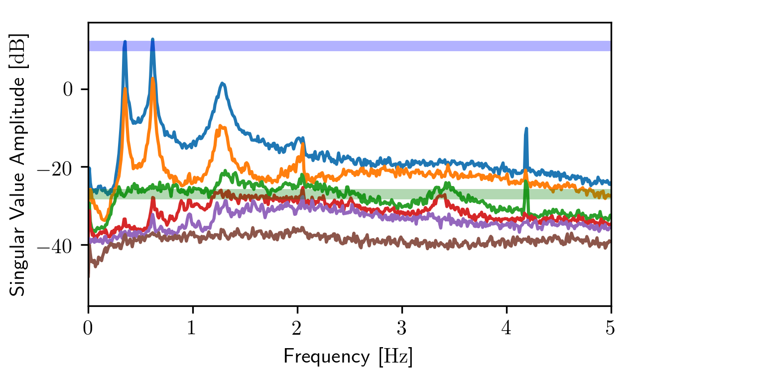
Singular-value PSD of a 30-minute acceleration record — Singular-value power spectral density of a 30-minute acceleration record. Peaks at approximately 0.35, 0.62, 1.3, 2.1, and 3.4 Hz correspond to the five bending mode pairs of the tower. *(Marwitz & Zabel, ISMA 2018.)*#

2. State caching for uninterrupted batch runs

from pathlib import Path

if not Path(prep_cache).exists():
    prep.save_state(prep_cache)
else:
    prep = PreProcessSignals.load_state(prep_cache)
    prep.sv_psd(n_lines, method='blackman-tukey', refs_only=False)

save_state() and load_state() allow the pipeline to resume after interruptions without recomputing the correlation functions. The same pattern applies to VarSSIRef and StabilCluster.

3. Identification

from pyOMA.core.VarSSIRef import VarSSIRef

modal = VarSSIRef.init_from_config(ssi_config_file, prep)
modal.save_state(modal_cache)

init_from_config() reads block-line count, model order range, and other SSI parameters from a plain-text config file, keeping tuning parameters separate from the pipeline code.

4. Automated stabilization

from pyOMA.core.StabilDiagram import StabilCluster

stabil = StabilCluster(modal, prep)
stabil.calculate_soft_critera_matrices()
stabil.calculate_stabilization_masks()
stabil.automatic_clearing()
stabil.automatic_classification()
stabil.automatic_selection()

freqs, damping, shapes, orders, *_ = stabil.return_results()

The three-stage automated procedure — clearing spurious poles, grouping similar poles into clusters, and selecting the best representative per cluster — replaces the manual stabilization diagram review that would otherwise be required for every 30-minute window.

Result storage with xarray#

The output of return_results() is collected across time windows and stored as a sparse, self-describing NetCDF database using xarray:

import numpy as np
import xarray as xr

# Build a single-window Dataset from return_results() output
ds = xr.Dataset(
    {
        'frequency': (['time', 'mode'], freqs[np.newaxis, :]),
        'damping':   (['time', 'mode'], damping[np.newaxis, :]),
        # mode_shapes: (n_dofs × n_modes) → store per DOF if needed
    },
    coords={
        'time': [start_time],
        'mode': np.arange(len(freqs)),
    },
)
# Merge into the growing long-term database
ds.to_netcdf(result_db_path, mode='a')

Results are sparse along all three dimensions:

time — gaps from system downtime or discarded low-quality windows;
modes — modes that are not excited in a given window are simply absent;
channels — sensors that fail or are replaced introduce gaps in mode-shape data.

xarray’s coordinate-aware indexing and built-in NaN handling make it straightforward to select subsets (e.g. all windows above a minimum wind speed), compute rolling statistics, and generate scatter plots without manually aligning index arrays.

Observations from long-term monitoring#

Frequency tracking over time

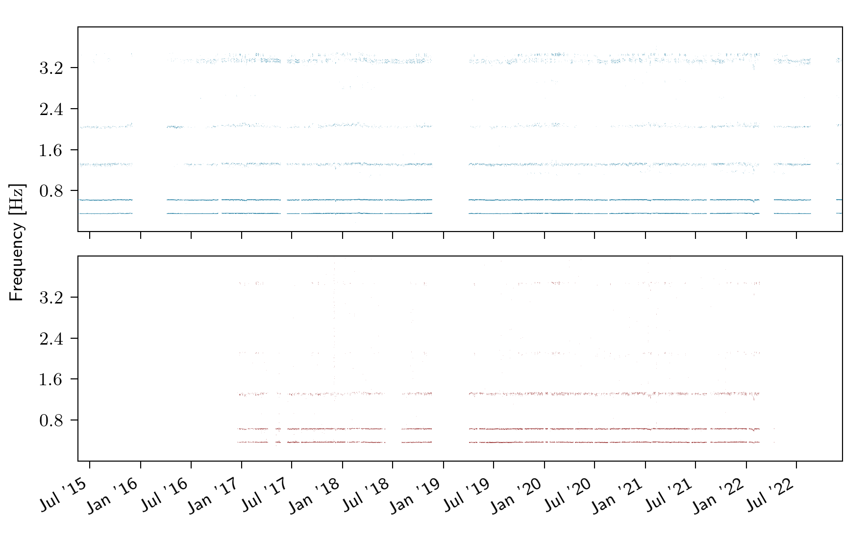
Identified natural frequencies over 7+ years (Jul 2015–Jul 2022). *Top*: accelerometer data (blue); *bottom*: FBG strain data (red). Five bending mode pairs are consistently identified; data gaps correspond to sensor maintenance periods. Strain-based identification starts in 2017 and reliably captures only the first three mode pairs due to the lower signal-to-noise ratio of strain measurements at higher frequencies. *(Zabel & Marwitz, EVACES 2023.)*#

Temperature–frequency relationship

Natural frequencies decrease approximately linearly with temperature across all mode pairs, as shown below. A decrease of about 2–3 % per 30 °C is consistent with decreasing elastic moduli at higher temperatures. The increased scatter below 0 °C is attributed to icing events that temporarily add mass to the structure and lower the natural frequencies by up to 10 % [EVACES2023].

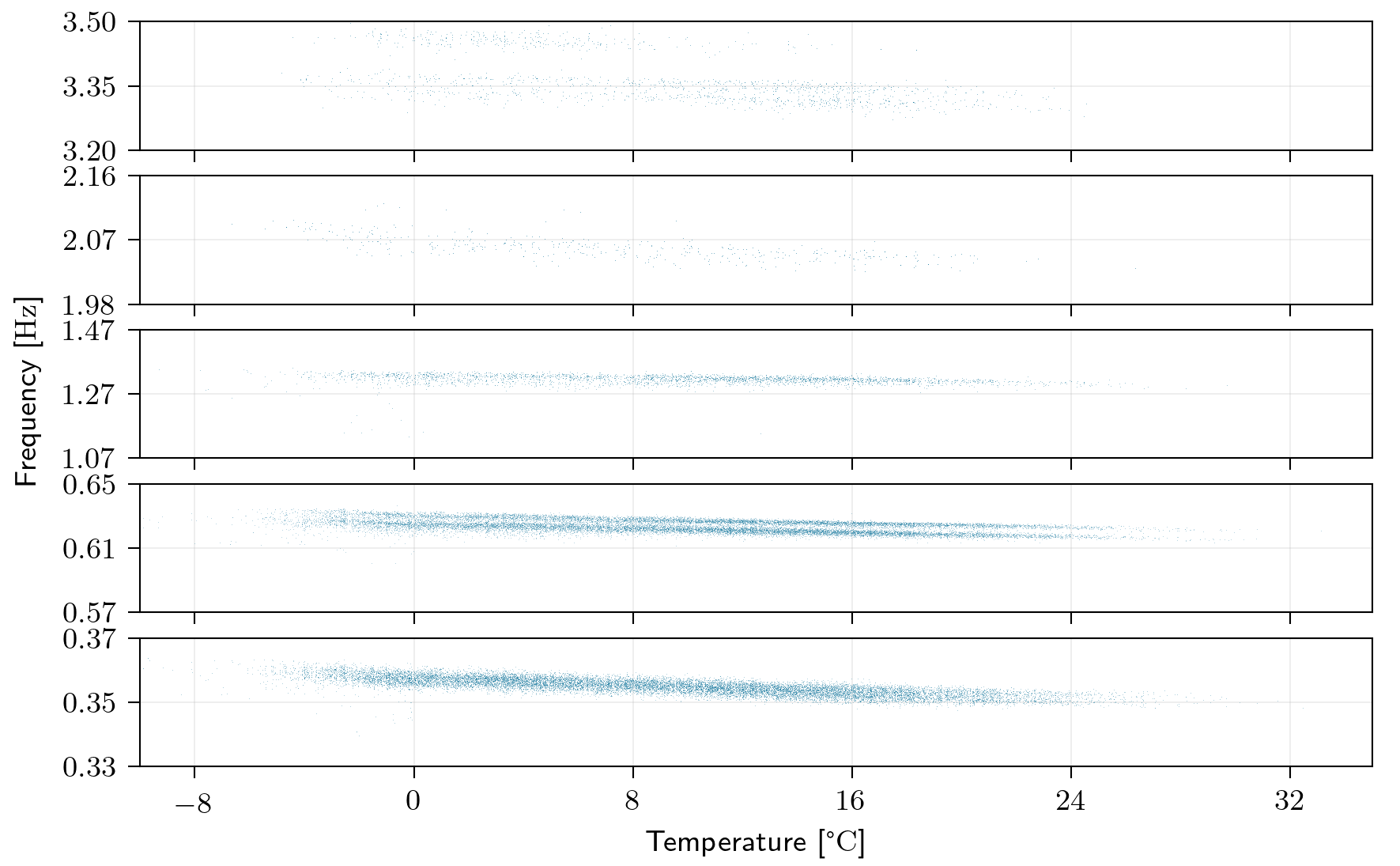
Identified natural frequencies vs. measured temperature for all five bending mode pairs (one panel per mode pair, bottom to top in ascending frequency order). *(Zabel & Marwitz, EVACES 2023.)*#

Wind speed–damping relationship

Modal damping ratios increase with wind speed, as shown for the first three mode pairs. The trend is attributed to aerodynamic damping and to stronger activation of the TMD at higher vibration amplitudes [ISMA2018].

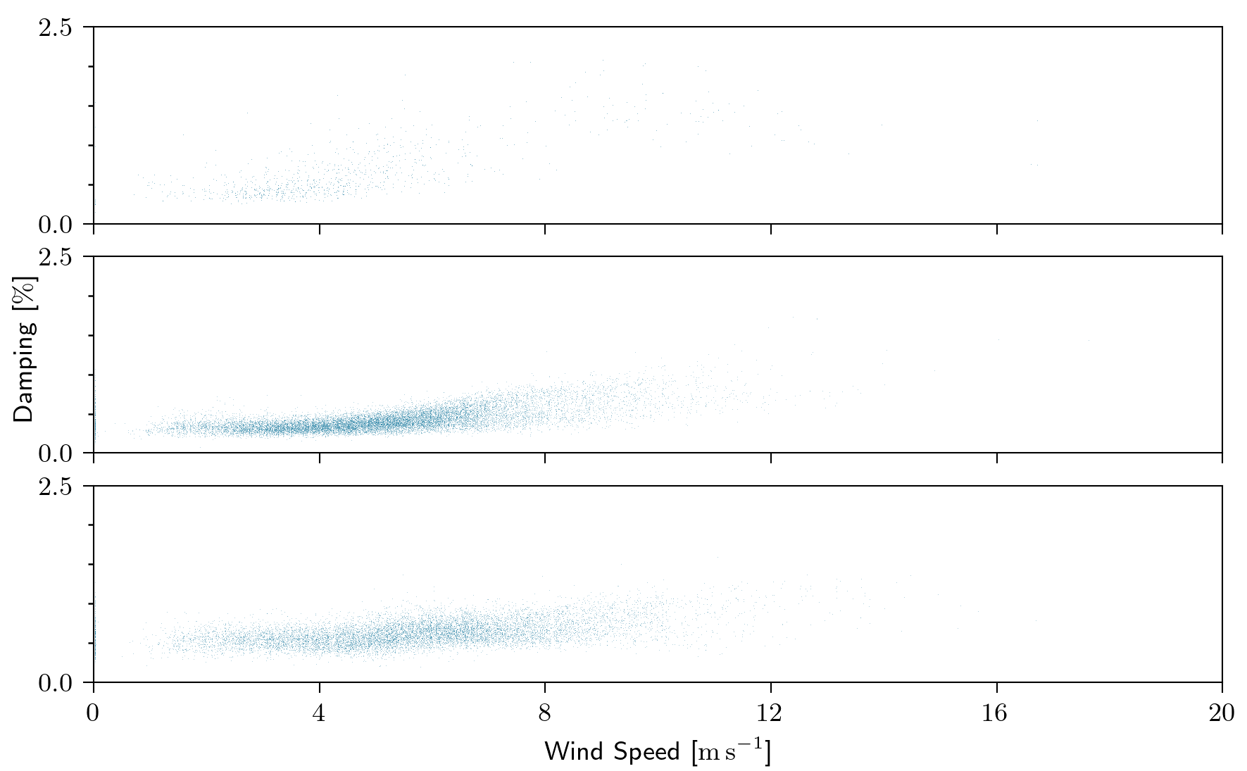
Identified modal damping ratios vs. wind speed — Identified modal damping ratios vs. 10-minute mean wind speed for three bending mode pairs (stacked panels). *(Zabel & Marwitz, EVACES 2023.)*#

References#

[ISMA2018] (1,2,3)

Marwitz, S. and Zabel, V. (2018). “Relations between the quality of identified modal parameters and measured data obtained by structural monitoring.” Proc. International Conference on Noise and Vibration Engineering (ISMA 2018), Leuven, Belgium.

[EVACES2023]

Zabel, V. and Marwitz, S. (2023). “Monitoring of the dynamic behaviour of a telecommunication tower.” Proc. Experimental Vibration Analysis for Civil Engineering Structures (EVACES 2023).